Explainability in Production AI Systems

In production, an unexplained prediction is often indistinguishable from a hallucination or a bug. When a loan officer asks "why was this applicant denied?", pointing to an F1 score isn't an answer. When a regulator audits your claims model, "the neural network said so" won't satisfy Article 13.

The business risk is straightforward: unexplained decisions erode trust, invite regulatory scrutiny, and make debugging nearly impossible. We've seen teams ship models that performed well on holdout sets but made decisions no one could justify to customers—or to themselves when things went wrong.

This piece covers what actually works in production: glass-box models that explain themselves, post-hoc methods with their real limitations, and the distinct challenge of explaining LLMs where traditional feature attribution doesn't apply. We focus on the trade-offs practitioners face—accuracy vs. transparency, real-time vs. batch explanations, generating explanations vs. presenting them to humans who aren't data scientists.

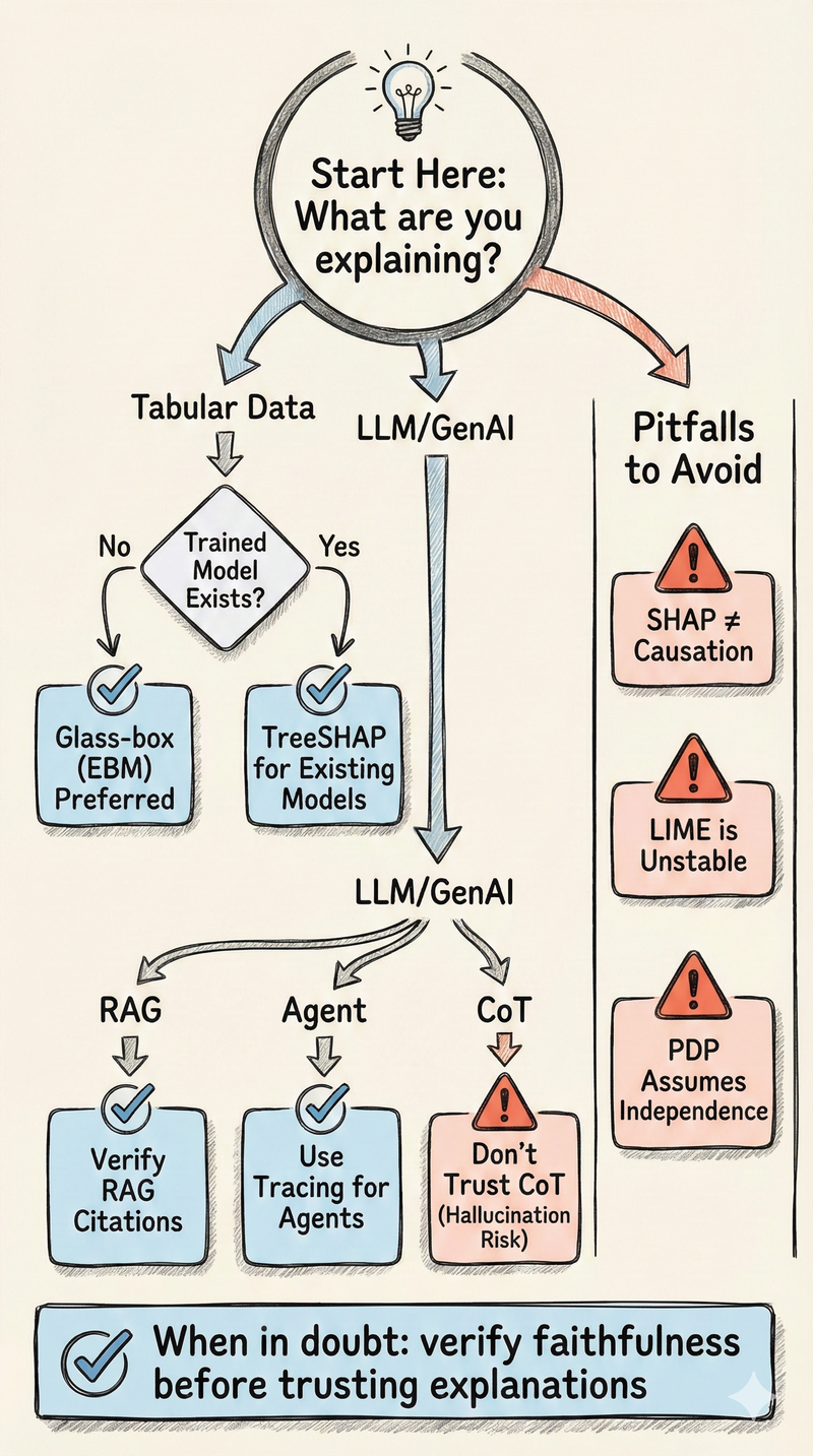
Explainability methods summary infographic — TL;DR: A visual summary of explainability methods and when to use each approach.

The Taxonomy: Three Trade-offs

Every explainability choice involves trade-offs. Understanding these helps you select the right approach—and know what you're giving up.

Five-tier stack showing interpretability levels — Interpretability Spectrum: From inherently interpretable to black box

Intrinsic vs Post-hoc is the most consequential choice. With intrinsic interpretability, the explanation is the model—no approximation, no risk of unfaithfulness. Post-hoc methods approximate a black-box model's behavior after training. Approximations can lie. The explanation might look plausible while completely misrepresenting the model's actual decision path. Global vs Local determines your audience. Global explanations describe overall model behavior—useful for model documentation, regulatory filings, and drift detection. Local explanations answer the customer's question: "why did I get this decision?" Most production systems need both, but they serve different stakeholders. Model-agnostic vs Model-specific is a speed-accuracy trade-off. KernelSHAP works on any model but has O(2^M) complexity—often prohibitively expensive for real-time inference. TreeSHAP exploits tree structure to compute exact Shapley values in polynomial time. If you're using XGBoost or LightGBM, always use TreeSHAP.

Glass-Box Models: Intrinsic Interpretability

When transparency is required, start with models that are interpretable by design. Here's the reality that many teams miss: on tabular data—the dominant data type in enterprise settings—the accuracy gap between glass-box models and black-box ensembles has largely closed.

Microsoft Research's benchmark across 13 classification tasks found EBMs matched or exceeded XGBoost on most datasets. Our experience confirms this. The cases where gradient boosting genuinely outperforms are rarer than the ML community assumes, and often the margin doesn't justify the interpretability debt.

Linear and Logistic Regression

The foundational interpretable models. The model calculates predictions as a weighted sum of input features:

Prediction = β₀ + β₁x₁ + β₂x₂ + ... + βₚxₚ

Each coefficient βⱼ directly quantifies how a one-unit change in feature xⱼ affects the prediction. In logistic regression, exp(βⱼ) gives the odds ratio—directly interpretable as "this factor increases odds by X%."

Strengths: Complete transparency. No approximation. Fast inference. Well-understood statistical properties with confidence intervals and hypothesis tests built in. Limitations: Assumes linear relationships and feature independence. You must manually specify interactions. When features are correlated (multicollinearity), coefficients become unstable—you can't disentangle individual feature effects, and small data changes cause large coefficient swings. Use case: Strong baselines. Domains where linear approximation is sufficient or legally required. Situations requiring statistical inference.

Generalized Additive Models (GAMs) and Explainable Boosting Machines (EBMs)

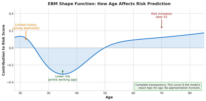
GAMs extend linear models by allowing non-linear relationships while preserving additive structure:

Prediction = f₁(x₁) + f₂(x₂) + ... + fₚ(xₚ)

Each shape function fⱼ can capture arbitrary non-linear patterns, but contributions remain additive—you can visualize each feature's effect independently.

Explainable Boosting Machines (EBMs) are Microsoft Research's implementation using gradient-boosted trees to learn each shape function. Key innovations:

Round-robin training mitigates collinearity effects
Automatic pairwise interaction detection
Competitive accuracy with XGBoost/LightGBM on tabular data

Neural Additive Models (NAMs) use small neural networks for each shape function, combining deep learning's expressiveness with GAM interpretability. Interpretation: Plot each shape function to see exactly how the model responds to that feature across its range. For local predictions, read off each feature's contribution and sum them. No approximation involved.

EBM Shape Function: Income effect on loan approval probability — Example EBM shape function showing how income contributes to loan approval probability. The relationship is fully transparent—no approximation required.

When to use: Tabular data where both accuracy and transparency matter. Regulated industries. Any setting where you need to document model behavior for auditors.

Post-Hoc Methods: Explaining Black Boxes

When you must use a black-box model (neural networks for images/text, or ensemble methods that outperform on your specific task), post-hoc methods provide approximate explanations. Understand their assumptions and failure modes.

SHAP (SHapley Additive exPlanations)

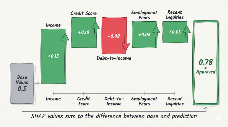
SHAP provides local feature attributions grounded in cooperative game theory. Each feature's SHAP value represents its average marginal contribution to the prediction across all possible feature combinations.

Key properties (unique among attribution methods):

Local accuracy: SHAP values sum to the difference between prediction and baseline
Consistency: If a feature's contribution increases in a new model, its SHAP value won't decrease
Missingness: Features with no effect get SHAP value of zero

Variants matter:

2x2 positioning map for explainability methods — Explainability Methods: Positioning map by fidelity and comprehensibility

TreeSHAP is the gold standard for tree-based models (XGBoost, LightGBM, Random Forest). It computes exact Shapley values in polynomial time by exploiting tree structure. Use this when working with gradient boosting. KernelSHAP is model-agnostic but has critical limitations. It uses permutation-based estimation that **assumes features are independent**. With correlated features, it generates unrealistic data combinations (e.g., a 25-year-old with 30 years of work experience), producing misleading attributions. The background dataset choice also affects results—different backgrounds yield different SHAP values. Operational reality: KernelSHAP is often prohibitively expensive for real-time inference. Most production systems run SHAP asynchronously—generating explanations offline for audit logs, compliance reports, or batch analysis, not inline for every customer interaction. TreeSHAP is faster but still adds latency; measure it against your SLA before promising real-time explanations. A common mistake: Teams treat SHAP values as causal drivers. They are not. SHAP measures predictive contribution—correlation suitable for understanding predictions, not for intervention. "Income has high SHAP value" means income helps predict the outcome, not that raising someone's income would change the decision. Conflating these leads to misguided "what should I change?" advice.

SHAP Waterfall: Feature contributions to a single prediction — SHAP waterfall plot showing how each feature contributes to pushing a prediction above or below the baseline. Red bars increase the prediction, blue bars decrease it.

LIME (Local Interpretable Model-agnostic Explanations)

LIME explains individual predictions by fitting a local linear model around the instance:

Generate perturbed samples near the instance
Get black-box predictions for perturbations
Fit weighted linear regression (weights decrease with distance)
Return linear model coefficients as feature importances

Critical limitation: LIME is unstable. Explanations are sensitive to:

Kernel width (defines "local" neighborhood)
Number of perturbations
Random seed

Different runs can produce contradictory explanations for the same prediction. Research has demonstrated "scaffolding attacks" where biased models can be wrapped to fool LIME into producing innocent-looking explanations. When LIME works: Quick intuition for individual predictions. Situations where you need model-agnostic explanations and SHAP is too slow. Always verify stability by running multiple times.

Anchors

Anchors provide explanations as IF-THEN rules: "IF income > $80K AND employment_years > 5, THEN loan approved (with 95% precision)."

Unlike SHAP/LIME which assign weights to all features, Anchors identifies a minimal sufficient condition. The rule's " coverage" metric indicates how broadly it applies.

When to use: When you need human-readable decision rules. Compliance contexts where "sufficient conditions" are more useful than "feature weights." Debugging specific prediction patterns.

Counterfactual Explanations

Counterfactuals answer a different question than feature attribution: "What would need to change for the decision to flip?"

Instead of "income contributed -0.3 to your score," a counterfactual says: "If your debt had been $5,000 lower, you would have been approved." This is often more actionable—and more legally defensible—than SHAP values.

Key properties:

Actionable: Identifies minimal changes to flip the decision
Legally relevant: Many regulations require telling customers what would change the outcome
Intuitive: Non-technical stakeholders understand "if X then Y" better than feature weights

Implementation: Libraries like Microsoft's DiCE (Diverse Counterfactual Explanations) generate multiple diverse counterfactuals, avoiding the trap of suggesting unrealistic single-point changes. Limitation: Counterfactuals can suggest changes to immutable features (age, protected characteristics). Production implementations need constraints to exclude these. Also, counterfactuals describe the decision boundary, not the model's reasoning—useful for customers, less so for model debugging.

Global Effect Plots: PDP vs ALE

Partial Dependence Plots (PDP) show average model response to a feature by averaging out the effects of other variables. Simple to compute and interpret. Fatal flaw: PDP assumes feature independence. It averages predictions over unrealistic feature combinations—asking " what if we changed income while holding all else constant?" even when income correlates strongly with education or job type. With correlated features (nearly universal in real data), PDP can be misleading. Accumulated Local Effects (ALE) fix this by computing effects in local windows conditional on the data distribution. ALE avoids unrealistic combinations. Recommendation: Default to ALE for global feature effects. Use PDP only when features are genuinely uncorrelated ( rare).

Verification: Testing Explanation Quality

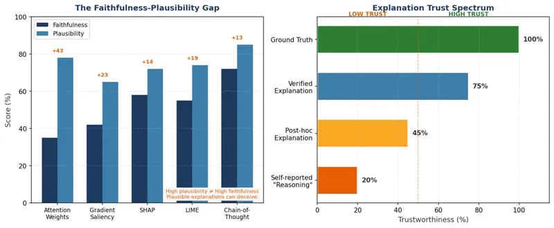
Post-hoc explanations can be wrong. Before trusting them for decisions or compliance, verify faithfulness and stability.

Faithfulness Tests

Do the "important" features actually matter to the model?

Deletion test: Remove features ranked as most important. Does prediction confidence drop significantly? If not, the explanation identified the wrong features. Sufficiency test: Keep only the top-k important features, mask everything else. Can you recover the prediction? If not, the explanation missed necessary features. Perturbation test: For CoT rationales, edit a reasoning step. Does the answer change? If the answer is stable despite rationale changes, the rationale was post-hoc fabrication.

Stability Tests

Resampling: Generate explanations with different background datasets or random seeds. High variance indicates unreliable explanations. Input perturbation: Make small, semantically irrelevant changes to input. Stable explanations shouldn't flip dramatically.

Adversarial Testing

Scaffolding attacks: Attempt to wrap your model in a deceptive layer that fools the explainer. If successful, your explanation method is vulnerable. This is red-teaming for XAI.

Drift Detection via Explanations

Explainability isn't just for point-in-time decisions—it's a powerful drift monitoring tool. If the top feature for " Loan Approval" suddenly shifts from "Income" to "Zip Code," you have a problem. Either your data distribution changed dramatically, or the model is picking up a spurious correlation you need to investigate.

What to monitor:

Feature importance rankings: Track global SHAP importance over time. Significant shifts warrant investigation.
Contribution distributions: If a feature's contribution distribution changes shape, something shifted.
Explanation clusters: Do explanations for different prediction outcomes still separate cleanly?

This provides a different lens than traditional drift detection (input distribution monitoring). Explanation-based monitoring catches cases where inputs look similar but the model's decision logic has shifted.

For comprehensive coverage of drift detection, monitoring infrastructure, and production ML operations, see LLM Application Lifecycle.

Explaining LLMs, RAG, and Agents

Traditional feature attribution doesn't transfer to generative AI. These systems require different approaches.

Chain-of-Thought: Plausibility ≠ Faithfulness

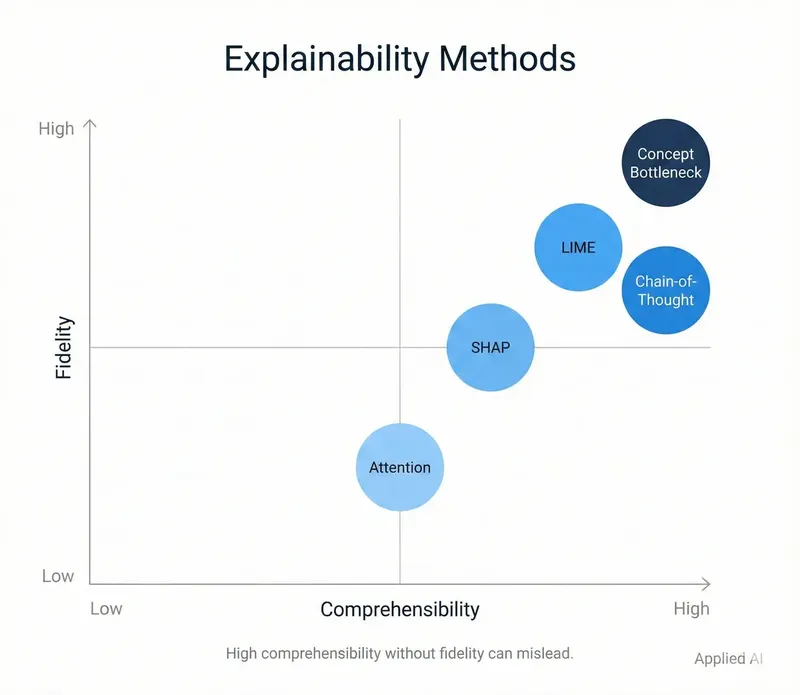
LLMs can generate step-by-step reasoning that improves task performance. But these rationales are often unfaithful —they don't reflect actual model computation.

Research from Anthropic shows models frequently:

Generate plausible reasoning that ignores the actual cause of their answer
Fail to disclose reliance on biased hints in prompts
Produce different rationales for the same underlying computation

Policy for production systems: Treat CoT as a UX feature that aids user comprehension, not as ground-truth explanation for audit purposes. For tasks requiring genuine auditability, decompose reasoning into deterministic code execution rather than LLM generation.

RAG Citations: The Faithfulness Problem

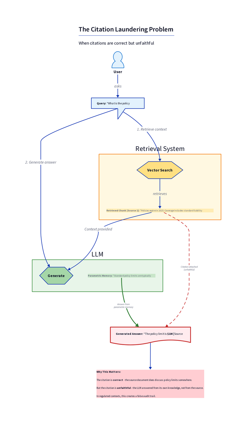
This is subtle but critical for anyone building generative AI. RAG systems cite source documents, and those citations can be correct while being unfaithful.

Correctness vs Faithfulness:

Correct citation: The cited document supports the claim
Faithful citation: The model actually used the document to generate the answer

These are not the same. Studies find up to 57% of RAG citations lack faithfulness—the model generated the answer from parametric memory, then attached a retrieved document that happened to support it. The citation looks legitimate, but the document didn't inform the answer.

We call this citation laundering: the model "launders" its internal knowledge through an external source, creating a false audit trail. In regulated contexts, this is a compliance failure even when the answer is factually correct.

Diagram showing faithfulness gap concept — Faithfulness Gap: When explanations don't match model behavior

Citation Laundering: How RAG citations can be correct but unfaithful — Citation laundering: the model generates an answer from parametric knowledge, then attaches a retrieved document that happens to support it—creating a false audit trail.

Detection approach: Remove the cited document from context and regenerate. If substantially the same answer appears, the citation was unfaithful. For production systems, implement entailment checks—verify that claims are actually entailed by cited text, not just topically associated with it.

Agent Observability: Traces, Not Explanations

Multi-step agents that use tools, query APIs, and take actions need different transparency mechanisms. Explaining a single prediction is insufficient when the system executes complex workflows.

Required infrastructure:

End-to-end tracing: OpenTelemetry with GenAI semantic conventions provides the foundation
Complete audit trail: Every prompt, every tool call, every intermediate decision captured
Reproducible execution logs: Forensic reconstruction must be possible

Concrete tooling options:

LangSmith: Purpose-built for LangChain applications, strong visualization
Arize Phoenix: Open-source, works with any framework, strong evaluation integration
OpenTelemetry + custom backend: Maximum flexibility, requires more setup
Weights & Biases Weave: Good for teams already using W&B

The explanation becomes the trace itself—a complete record of what the agent did and why. For compliance purposes, you need to answer: "Given the same inputs, can we reproduce the agent's decision path?" That requires capturing not just final outputs but all intermediate state. Cost reality: Full trace logging for high-throughput agents generates massive data volumes. Production teams often need sampling strategies—trace 100% of errors and edge cases, 1% of routine successes—to manage storage costs without losing the ability to debug failures.

Presenting Explanations: The Translation Layer

Generating explanations is only half the problem. The other half is presenting them to humans who aren't data scientists.

A raw SHAP force plot is confusing to a business user. A log-odds chart doesn't help a loan officer explain a decision to a customer. The technical artifact that satisfies an ML engineer is often a UX failure for everyone else.

UI patterns that work:

Confidence indicators: Visual cues (color bars, percentage displays) showing model certainty
Top-3 factors: Plain-language summary of the most influential features ("Your application was declined primarily

due to: high debt-to-income ratio, recent credit inquiries, short employment history")

Comparative framing: "Compared to approved applicants, your debt-to-income ratio is in the top 15%"
Drill-down capability: High-level summary for most users, detailed attribution available on demand

The translation challenge: Different stakeholders need different views. A compliance auditor wants the full SHAP breakdown. A customer wants actionable guidance. A loan officer needs enough to explain the decision in 30 seconds. Design for all three.

For document extraction, we've found that linking explanations to source evidence—letting reviewers click from "Age Limit: 65" to the exact PDF page and paragraph—dramatically increases trust. Abstract feature weights don't provide that grounding.

Production Case Study: Contract Intelligence Pipeline

To make this concrete: we built a document intelligence system for insurance contract analysis. The system extracted policy attributes—convertibility options, age limits, premium conditions—from decades of documents in inconsistent formats.

A black-box "throw an LLM at PDFs" approach wasn't acceptable. Stakeholders needed to understand every extraction. Regulators needed audit trails.

How we built explainability in: Evidence linking: Every extracted attribute tied to specific text spans. Not just "Age Limit: 65" but "Age Limit: 65, from Section 4.2, paragraph 3, lines 15-18." Reviewers click through to source PDF. Confidence-aware routing: Calibrated confidence scores determined workflow:

High confidence → auto-approved
Boundary cases → human review queue
Low confidence → manual extraction required

This focused expert attention on ambiguous cases rather than reviewing everything. Anti-hallucination validation: Regex-based checks confirmed extracted numbers appeared in supporting text. Negative assertions ("no convertibility clause") required evidence of absence—documented review of relevant sections. Boundary case surfacing: Records near decision thresholds surfaced proactively. Reviewers saw candidate text spans, compared to model output, adjusted labels. System learned from corrections.

The result: every decision traceable to source evidence. Not because we bolted on explanations after building the model, but because traceability was an architecture requirement from day one.

Practical Framework: Choosing Your Approach

Decision Matrix

Before Deployment Checklist

For post-hoc explanations:

[ ] Faithfulness tested (deletion, sufficiency)
[ ] Stability verified (resampling, perturbation)
[ ] Adversarial robustness assessed
[ ] Documentation suitable for audit

For LLM/RAG systems:

[ ] Citation faithfulness verification implemented
[ ] CoT treated as UX, not compliance artifact
[ ] End-to-end tracing operational

For agents:

[ ] Complete audit trail captured
[ ] Traces reproducible
[ ] Forensic reconstruction possible

Governance Alignment

XAI practices map directly to regulatory requirements:

Decision flowchart for explainability methods — Explainability Decision Framework: Choosing the right method

Explanation artifacts—shape function plots, faithfulness reports, trace exports—become compliance evidence. Organizations that generate and archive these artifacts systematically transform XAI from technical exercise into governance infrastructure.

Key Takeaways

Glass-box when possible: On tabular data, EBMs and GAMs often match black-box accuracy. The explanation debt you avoid is worth it. Know your method's assumptions: SHAP assumes feature independence (except TreeSHAP). PDP assumes feature independence. LIME is unstable. These aren't reasons to avoid them—they're reasons to verify them. Verify, don't trust: Post-hoc explanations can be unfaithful. Test faithfulness and stability before relying on them for decisions or compliance. LLMs are different: CoT isn't ground truth. RAG citations can be unfaithful. Agents need traces, not feature attributions. Build explainability in: Retrofit explanations are approximations at best. Design for transparency from the start when requirements demand it.

The organizations that get this right treat explainability as architecture, not afterthought. They select models appropriate to their transparency requirements. They verify explanation quality. They build audit infrastructure from day one. That's how you ship AI systems that stakeholders can interrogate, regulators can inspect, and teams can actually trust.

References

Caruana, R. et al. (2015). "Intelligible Models for HealthCare." KDD 2015.

Lundberg, S. & Lee, S. (2017). "A Unified Approach to Interpreting Model Predictions." NeurIPS 2017.

Mothilal, R.K. et al. (2020). "Explaining Machine Learning Classifiers through Diverse Counterfactual Explanations." FAT* 2020.

Molnar, C. (2022). Interpretable Machine Learning. https://christophm.github.io/interpretable-ml-book/

Nori, H. et al. (2019). "InterpretML: A Unified Framework for Machine Learning Interpretability." arXiv:1909.09223.

Ribeiro, M. et al. (2016). "Why Should I Trust You?: Explaining the Predictions of Any Classifier." KDD 2016.

Rudin, C. (2019). "Stop Explaining Black Box Machine Learning Models for High Stakes Decisions and Use Interpretable Models Instead." Nature Machine Intelligence.

Slack, D. et al. (2020). "Fooling LIME and SHAP: Adversarial Attacks on Post hoc Explanation Methods." AIES 2020.

Turpin, M. et al. (2023). "Language Models Don't Always Say What They Think: Unfaithful Explanations in Chain-of-Thought Prompting." NeurIPS 2023.