Beyond Response Models: Causal ML for Marketing

Marketing has a prediction problem. Not because we can't predict—modern machine learning excels at forecasting who will click, convert, or churn. The problem is that prediction is not causality.

A response model tells you which customers are likely to buy. What it doesn't tell you is which customers will buy because of your campaign. That distinction costs money. When you target "sure things"—customers who would have purchased anyway—you're paying for conversions you'd get for free. When discount campaigns reach buyers willing to pay full price, you cannibalize your margins. In subscription businesses, a poorly timed retention offer can remind customers to cancel a service they'd forgotten about.

This is where uplift modeling earns its place. Rather than predicting outcomes, it estimates causal effects: the incremental impact of your intervention on each customer's behavior. The question shifts from "who will convert?" to "who will convert because we contacted them?"

The difference shows up in ROI. Organizations implementing uplift modeling consistently report 15-40% improvements in campaign efficiency—not by finding more customers, but by avoiding wasted spend on the wrong ones.

The Correlation Trap

Traditional response models optimize for correlation. Train a classifier on historical campaign data, score customers by conversion probability, and target the top decile. This works if your goal is prediction accuracy. It fails when your goal is incremental lift.

The failure mode is subtle but expensive. Consider two customers, both with an 80% probability of converting:

Customer A: 80% with offer, 10% without offer → 70 percentage points of uplift
Customer B: 80% with offer, 80% without offer → 0 percentage points of uplift

A response model can't distinguish between them. Both get the same score. Both receive the campaign. But only Customer A generates incremental value. Customer B represents pure waste—you've paid to deliver an offer to someone who was already going to buy.

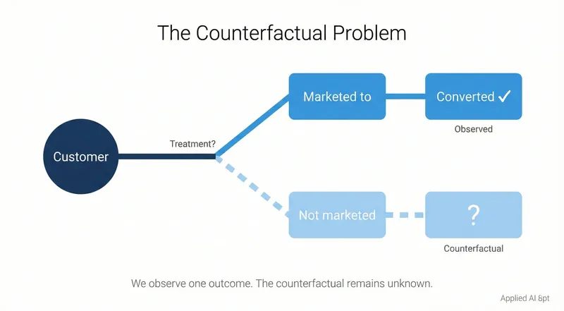
Uplift modeling makes this distinction by estimating the counterfactual: what would have happened without intervention? This requires moving from predictive modeling to causal inference.

The Fundamental Problem of Causal Inference: We never observe both potential outcomes for the same customer—you either sent them the offer or you didn't. You can't know what Customer B would have done without the offer because you sent it. This fundamental impossibility is why we need sophisticated methods (meta-learners, causal forests) that estimate individual-level effects from group-level comparisons.

The Counterfactual Problem: We observe one outcome (marketed to → converted). The counterfactual (no

Four Customer Personas: A Strategic Framework

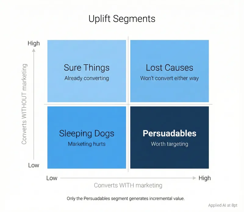
Uplift modeling segments customers not by demographics or behavior, but by how they respond to marketing interventions. This creates four distinct personas, each requiring a different strategy:

1. Persuadables (Target Aggressively)

These customers convert only if they receive your offer. Conversion probability jumps from low baseline to high with intervention. This is your target segment—the only group generating genuine incremental value.

Example: A price-sensitive shopper hesitating between your product and a competitor's. A 15% discount closes the deal. Without it, they go elsewhere.

Strategy: Concentrate all resources here. This is where campaign ROI comes from.

2. Sure Things (Exclude to Preserve Margins)

These customers convert regardless of whether you contact them. They're going to buy anyway, at full price, without prompting.

Example: A loyal subscriber up for renewal who values your service and has no intention of leaving. A retention discount just reduces your revenue.

Why this matters: In a mature SaaS business, sure things might represent 30-40% of your "high propensity" segment. Every dollar spent here is margin lost.

Strategy: Exclude them. Let them buy at full price.

3. Lost Causes (Exclude to Save Budget)

These customers won't convert no matter what you do. High discount, personalized outreach, premium support—none of it changes the outcome.

Example: A prospect researching enterprise software when your product is built for SMB. Wrong fit, wrong budget, wrong use case.

Strategy: Don't waste resources. Focus budget on persuadables.

4. Sleeping Dogs (Actively Avoid)

These customers have negative uplift. Your intervention makes them less likely to convert. This is the most dangerous segment.

Example: A satisfied customer who hasn't thought about canceling until your retention campaign reminds them they're paying for a service they rarely use. The email triggers a cancellation you would have avoided by staying silent.

Why this matters: In churn prevention campaigns, sleeping dogs can represent 5-15% of your target list. Contacting them actively destroys value.

A caveat on statistical significance: Negative uplift estimates often have high variance. Before labeling a customer segment as sleeping dogs, verify the effect is statistically significant—not just noise from small samples. A predicted -0.5% uplift might be statistical noise rather than true negative sentiment. Apply a confidence threshold (e.g., lower bound of 95% CI < 0) before suppression.

Strategy: Identify and suppress with confidence. Never contact customers with statistically significant negative uplift.

The business case for uplift modeling becomes clear when you quantify these segments. In a typical retention campaign:

30% persuadables (incremental value)
35% sure things (wasted discounts)
25% lost causes (wasted outreach)
10% sleeping dogs (value destruction)

A response model targets everyone with high P(convert). An uplift model targets only the 30% that matter.

Uplift Segments: 2x2 matrix showing the four customer personas—Sure Things, Lost Causes, Persuadable

When Uplift Modeling Earns Its Complexity

Uplift modeling adds methodological overhead. You need experimental data, specialized algorithms, and uplift-specific evaluation metrics. That overhead only makes sense in specific contexts.

High-Value Scenarios

Costly interventions: When the cost per treatment is substantial—outbound sales calls, high-value discounts, physical direct mail—the penalty for targeting non-responsive segments becomes prohibitive. A $50 discount offered to sure things who'd pay full price costs you $50 per person in pure margin loss.

Scarce resources: Budget constraints make targeting decisions zero-sum. Every dollar spent on lost causes is a dollar not spent on persuadables. Uplift modeling provides a principled framework for allocation under scarcity.

Churn prevention: Subscription businesses carry inherent risk of waking sleeping dogs. A poorly timed retention offer can trigger cancellations. Uplift modeling identifies these negative-effect customers before you contact them.

Mature markets: When organic growth slows and customer acquisition becomes expensive, identifying pockets of persuadable customers provides one of the few levers for incremental gains.

When to Use Standard Response Models

Uplift modeling is overkill when:

Treatment costs are negligible (low-cost email campaigns)
You have budget to contact everyone anyway
Negative effects are implausible
You lack proper experimental data (more on this below)

The decision comes down to economics. If the cost of mis-targeting (wasted discounts, sleeping dog activation) exceeds the cost of building an uplift model, the investment pays for itself. For a retention campaign offering $100 discounts to 100,000 customers, avoiding just 10% waste saves $1M.

Methods Overview: From Simple to Robust

Uplift modeling draws from causal inference, a field with strong theoretical foundations but complex methodology. The practical question for marketers: which method should you use?

Meta-Learners: Flexible and Practical

Meta-learners adapt standard machine learning models to estimate causal effects. You can use standard base learners—such as LightGBM, Random Forests, or Neural Networks—without modifying their objective functions.

T-Learner (Two-Model Approach) Train two separate models: one on treatment group data, one on control group data. Estimate uplift as the difference in their predictions.

When to use: Quick POCs and baselines. Often "good enough" for V1 implementations. Strengths: Conceptually straightforward. Works with any ML algorithm. Limitations: Can have high variance with small samples. Each model optimizes for prediction, not causal effect estimation, which can lead to noisy uplift estimates.

X-Learner A more sophisticated variant that uses the full dataset twice and weights estimates by propensity scores. Performs better when treatment and control groups are imbalanced (common in observational data).

When to use: Moderate sample sizes (5K-50K) with imbalanced treatment/control groups. Strengths: More data-efficient than T-Learner. Handles imbalanced data well. Limitations: More complex to implement.

R-Learner Based on semi-parametric theory, the R-Learner isolates the causal effect from main effects through "orthogonalization"—a two-step process that first removes the noise of main effects (baseline outcome and propensity to be treated) to isolate the treatment signal. It directly optimizes for the uplift function rather than outcome prediction.

When to use: When you need maximum robustness and can invest in implementation complexity. Strengths: Strong theoretical properties. Robust to errors in nuisance models (outcome and propensity score). Doubly robust. Limitations: Most complex meta-learner to implement correctly.

Practitioner guidance: Start with T-Learner as a baseline. Upgrade to X-Learner if you have imbalanced groups. Use R-Learner when you need maximum robustness and have the implementation bandwidth.

Causal Forests: State of the Art for Tabular Data

Causal Forests adapt random forests specifically for heterogeneous treatment effect estimation. Instead of splitting nodes to minimize prediction error, they split to maximize treatment effect heterogeneity.

Key innovation: "Honest" estimation separates the data used to build tree structure from the data used to estimate effects within leaves. This prevents overfitting and enables valid confidence intervals.

When to use: Large samples (50K+), complex heterogeneity, when you need explainability for regulators (e.g., via SHAP values), or when confidence intervals matter.

Strengths:

Theoretical guarantees (consistency, asymptotic normality)
Automatic non-linearity and interaction detection
Interpretable through SHAP values
Confidence intervals for individual-level estimates

Limitations:

Requires large samples (thousands, not hundreds)
Computationally intensive
"Honesty" reduces sample efficiency

Implementation: Use the `grf` package in R or `CausalForestDML` in Python's EconML library.

Empirical performance: In benchmarks on marketing datasets, Causal Forests typically match or exceed meta-learners on AUUC (Area Under Uplift Curve), particularly when sample sizes are large and treatment effects are genuinely heterogeneous.

Decision Matrix

Method	Sample Size Need	Best For	Implementation Complexity
T-Learner	Medium	Quick baseline, simple campaigns	Low
X-Learner	Medium	Imbalanced data, modest sample	Medium
R-Learner	Medium	Maximum robustness needed	High
Causal Forest	Large	Complex heterogeneity, need confidence intervals	High

For most marketing applications with standard RCT data: Causal Forests for large samples (50K+), X-Learner for moderate samples (5K-50K).

The Experimental Data Requirement

The primary barrier to uplift modeling isn't algorithmic—it's the data requirement. You need data from a properly randomized experiment.

Uplift modeling estimates a causal effect. Causal inference requires comparing outcomes under treatment vs. no treatment. To make that comparison valid, treatment assignment must be random—independent of customer characteristics that also affect the outcome.

An observational analysis won't work. If you assign high-value customers to receive retention offers and low-value customers to receive nothing, any difference in outcomes conflates two effects: the treatment effect and the pre-existing difference between groups. You can't disentangle them without strong, untestable assumptions.

The Gold Standard: Randomized Holdout

The operational requirement is straightforward but often politically difficult:

Random assignment: Allocate customers to treatment vs. control by random draw, not by business rules or targeting scores
Clean control group: The control group receives nothing—no alternative campaign, no contamination from other marketing touches
Sufficient sample size: Enough observations in both groups to detect the expected effect size

In practice, this means maintaining a persistent global holdout—a randomly selected subset of your customer base that never receives marketing communications. This group serves as your counterfactual baseline.

Many marketing organizations resist this. The pushback is predictable: "Why would we intentionally not market to 10-20% of our customers?" The answer: because without that holdout, you have no way to measure incrementality. You're flying blind.

Minimum Viable Experiment

For a binary outcome (convert/don't convert) with:

Baseline conversion rate: 5%
Expected uplift: 2 percentage points (from 5% to 7%)
Standard A/B test parameters (80% power, 5% significance)

You need roughly 3,800 customers per group—7,600 total. For smaller effects or lower base rates, multiply accordingly. A 0.5 percentage point uplift at 2% baseline requires 60,000+ per group.

This sample size requirement often surprises practitioners used to response modeling, where you can build decent models on thousands of records. Uplift modeling is harder because you're estimating a difference in probabilities, which has inherently higher variance than estimating a probability itself.

What If You Don't Have RCT Data?

If you lack experimental data, you have three options:

Run an experiment now (recommended): Design a proper RCT, run it for 2-4 weeks, collect the data. This is almost always the right answer.

Quasi-experimental methods (advanced): If you have observational data with plausibly random treatment assignment (e.g., geographic rollouts, capacity constraints that create natural experiments), methods like Difference-in-Differences or Regression Discontinuity may work. These require strong domain knowledge and careful validation.

Don't do uplift modeling (honest): If you can't get experimental data and quasi-experimental assumptions don't hold, stick with response models. A biased uplift model is worse than no uplift model.

Evaluation: Why AUC Doesn't Work

You cannot evaluate an uplift model with standard classification metrics. AUC, accuracy, precision, recall—all measure predictive performance on observed outcomes. Uplift modeling predicts unobserved counterfactual differences.

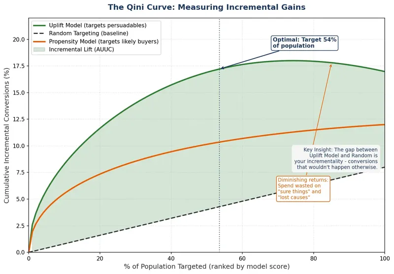
The Uplift Curve (Qini Curve)

The standard evaluation tool is the uplift curve:

Score all validation set customers with your uplift model
Rank them by predicted uplift (highest to lowest)
Divide into deciles
For each decile, calculate cumulative incremental gain:

`(Conversions_treatment / N_treatment) - (Conversions_control / N_control) × N_treatment`

Plot cumulative gain (y-axis) vs. proportion of population targeted (x-axis)

A good model shows steep early gains—the top deciles contribute most of the incremental lift. A bad model looks like a diagonal line (no better than random).

Area Under Uplift Curve (AUUC): Scalar summary metric. Larger is better. Use this for model comparison and hyperparameter tuning.

Economic interpretation: At any point on the curve, you can calculate expected incremental profit:

The Qini Curve: Measuring Incremental Gains. Shows uplift model outperforming random targeting and p

Incremental profit = (Incremental conversions × Value per conversion) - (Customers targeted × Cost per treatment)

This lets you set targeting thresholds based on ROI rather than arbitrary decile cutoffs. Target everyone with positive expected profit; exclude everyone else.

Out-of-Time Validation

Use chronological train/test splits, not random splits. Train on January data, validate on February data. This mimics production deployment and catches concept drift (changing customer behavior over time).

Random cross-validation inflates performance estimates by leaking information across time boundaries. In marketing, seasonality and trend matter. Validate on future data.

Implementation Checklist

Before starting an uplift modeling project:

Data Foundation

[ ] Access to RCT data with clean treatment/control split
[ ] Minimum 5,000 observations per group (preferably 10K+)
[ ] Control group truly received no treatment (no contamination)
[ ] Features captured strictly before treatment assignment (preventing data leakage)

Business Context

[ ] Treatment cost quantified (including soft costs)
[ ] Outcome value quantified in dollars
[ ] Budget constraints or capacity limits defined
[ ] Stakeholder buy-in for targeting restrictions (excluding high-propensity customers)

Technical Capabilities

[ ] Team familiar with causal inference concepts
[ ] Access to uplift modeling libraries (CausalML, EconML, or grf)
[ ] Ability to deploy models and refresh predictions
[ ] Monitoring infrastructure for model drift

Initial Approach

[ ] Start with T-Learner baseline
[ ] Evaluate on AUUC, not AUC
[ ] Validate on out-of-time data
[ ] Calculate economic value at different targeting thresholds
[ ] Test deployment on small segment before full rollout

Case Study: SaaS Retention Campaign

A B2B SaaS company with 200,000 subscribers ran annual retention campaigns offering 20% discounts to customers flagged as high churn risk.

Previous approach (response model):

Logistic regression predicting P(churn)
Target top 20% by churn probability (~40,000 customers)
Offer: 20% discount for annual renewal
Cost: $100/customer in margin loss
Total cost: $4M

Uplift modeling approach:

60/40 RCT split over 3 months (historical data)
Causal Forest model estimating uplift
AUUC: 0.087 (vs 0.031 for T-Learner baseline)

Segmentation results:

18% persuadables (incremental value from offer)
37% sure things (would renew without discount)
38% lost causes (won't renew regardless)
7% sleeping dogs (offer triggers churn)

Deployment strategy:

Target only customers with predicted uplift > 5 percentage points
This identified 22% of the original target list (8,800 customers)
Exclude predicted negative uplift entirely

Results:

Discount cost reduced from $4M to $880K (78% reduction)
Incremental retention: 510 customers (vs. 380 with response model)
ROI: 2.9x (vs. 0.9x with response model)

The key insight: 37% of the "high-risk" segment were sure things who would have renewed at full price. The response model couldn't identify them. The uplift model could.

Common Pitfalls

Contaminated control groups: If your control group receives alternative campaigns, you're measuring relative lift between two treatments, not absolute lift vs. doing nothing. This systematically underestimates true incrementality.

Confusing uplift with propensity: Uplift models predict `P(Y=1|T=1) - P(Y=1|T=0)`. Propensity models predict `P(Y=1|T=1)`. These are different quantities. Don't evaluate uplift models with propensity metrics.

Ignoring costs: An uplift model tells you who responds most to treatment. It doesn't tell you whether that response is profitable. Always incorporate treatment cost and outcome value into targeting decisions.

Sleeping dog denial: Many practitioners assume negative effects don't exist in their business. Test this assumption. In retention campaigns, we routinely find 5-15% negative uplift. Ignoring this segment destroys value.

Over-tuning on AUUC: Uplift models can have high variance. A model that looks great on one validation fold may perform poorly on another. Use multiple folds or bootstrap samples to assess stability.

When Uplift Modeling Pays Off

The economic threshold is straightforward. Uplift modeling makes sense when:

(% sure things + % sleeping dogs) × Treatment cost × Target volume > Cost of model development

For a retention campaign:

40% sure things + sleeping dogs
$100 treatment cost
40,000 target volume
Potential waste: $1.6M/year

If building the uplift model costs $200K in data science time and infrastructure, the ROI is 8x in year one. For ongoing campaigns, the ROI compounds.

The methodology is complex. The business case is simple: avoid wasting money on customers who don't need your intervention.

Beyond Marketing: Cross-Functional Applications

While this article focuses on marketing, uplift modeling applies wherever interventions have costs and you need to optimize resource allocation:

Customer success: Which at-risk accounts benefit from high-touch support vs. self-service resources?
Pricing: Which customers are price-sensitive enough to churn on a price increase but loyal enough to stay with a discount?
Product recommendations: Which users engage more when shown personalized content vs. default feeds?
Policy interventions: Which citizens respond to nudges vs. mandates in public health campaigns?

The unifying requirement: you need to measure causal effects, not just correlations. When you have that need, uplift modeling provides the framework.

Getting Started

If you're convinced uplift modeling fits your use case:

Design an experiment: Random assignment, clean control, sufficient sample size
Run it for 2-4 weeks: Collect outcome data with enough time to observe effects
Start with T-Learner: Build a simple baseline using LightGBM or Random Forest
Evaluate on uplift curves: Plot AUUC, compare to random targeting
Calculate economic value: Translate uplift scores to expected profit at different thresholds
Pilot deployment: Test targeting policy on 10-20% of next campaign
Monitor and iterate: Track in-production performance, retrain regularly

The hardest part isn't the modeling—it's convincing stakeholders to leave money on the table by not marketing to high-propensity customers. The sure things look attractive. They have high predicted conversion rates. Excluding them feels wrong.

But that's exactly the point. Response models confuse high propensity with high incrementality. Uplift models separate them. Once you see the difference in ROI, the strategic shift becomes obvious: target incremental value, not predicted outcomes.